7.2 Generating physical vulnerability curves

Flood damage assessment can be performed in a semi-quantitative way. It means that the damages have to be quantified per each category of asset according to the aggregation level chosen for the assessment. Stage-damage functions represent the most effective solution in relating flood parameters to damage in flood damage assessment models (Krzysztofowicz and Davis, 1983a; Krzysztofowicz and Davis, 1983b).

Stage-damage functions are mathematical functions that express the relation between the degree of the damage and flood parameters: the figure below shows two types of stage-damage functions. 

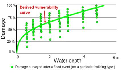
Empirical methods are either based on damage data from historical hazard events, or on expert opinion.  The figure illustrates the use of damage surveys for the generation of vulnerability curves. The green dots shows the damage surveyed after a flood event for a particular building type. The range of damage results for the same intensity depends on the definition of the building types. If the building types are very similar, also the degree of damage that will be observed is more similar than for buildings that have a large variation within the group.The damage can be assessed with remote sensing data, for example, video images, oblique photographs and high resolution satellite imagery.

Before you start:	Use case Location:	Uses GIS data:	Authors:
Read section 5.3 of the Methodology book	Generic location on one of the islands	Yes, it requires a point file with flood damage survey data	Cees van Westen and Nanette Kingma

 

Introduction:

In the following steps we will learn how to build depth-damage functions for different building types. Depth-damage functions are a particular type of stage-damage functions that relate the loss/damage to flood water depth. Stage-damage functions quantify, through mathematical equations, how the damage rate varies with the variation of flood parameter; therefore they are applied in semi-quantitative flood damage assessment. They express the vulnerability of each element at risk to a certain parameter when affected by a flood event. The elements at risk are grouped in classes according to the degree of aggregation at which we want to perform the risk assessment. Elements at risk can refer to building types (one storey wood buildings, single houses from bricks in mud, multiple storey reinforced concrete buildings, etc.) or they can be aggregated into residential, commercial, industrial and agricultural units. In figure X.X, two types of stage-damage functions are shown: the two graphs on top relate the damage expressed in percentage for residential concrete houses to water depth; the other two graphs represent the relation between the damage and the duration of flood for different types of crops (Dutta et al., 2003)

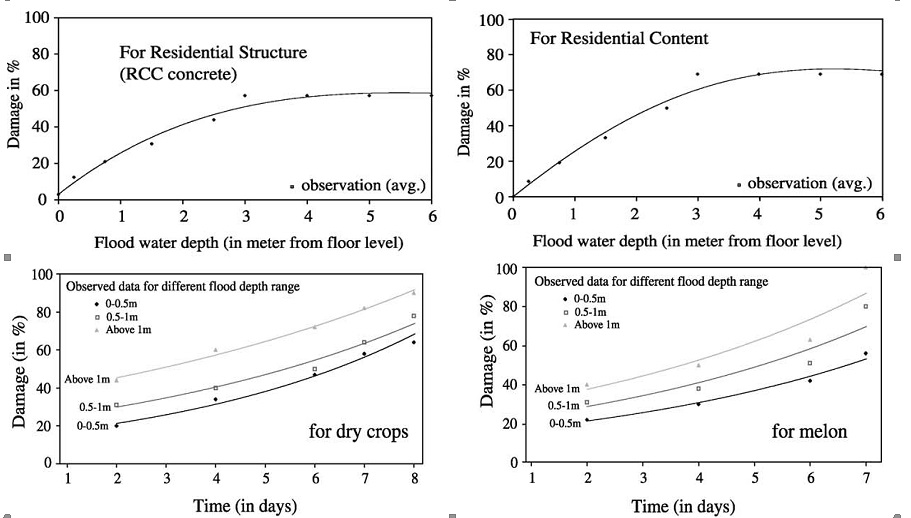
Figure: Examples of vulnerability curves or stage damage curves for residential structures and residential content. The lower graphs show curves of different waterdepth and time as a function of damage for crops (Dutta et al.,2003) . 

Stage-damage functions can be extracted following two strategies: the first consist of calculating the functions on the basis of historical flood damages data; the second is the calculation of functions from analysis based on: expert knowledge based estimations on assets classes, questionnaire surveys, and the aggregation of that information to assets units or landcover classes. In this case they are called synthetic stage damage functions.

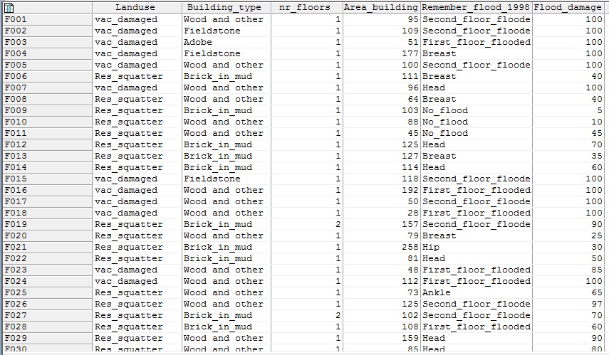
We will gather the information needed to build the functions from the surveys realized during PGIS activities. The data collected are stored in a table called PGIS_Survey; the data are related to landslides and flood hazards, but we will use only the data related to the three historic floods occurred in 1993, 1998, 2008. The table shows 200 locations of interviews; each one related to one building; the IDs F001 to F100 regard the flood events; every record is an average of the answers and estimations of all the single families that live or were living during the disasters in that particular building. The questions regarded flood depth, caused damage, behavior of people, cars, and buildings in relation to the strength of the flood. The answers are expressed by "codes"  easily comprehensible for the population and meaningful for the further calculations.  

The collection of local knowledge is very important in risk assessment. Local communities are the most important stakeholder in risk assessment, and are often the ones that are most at risk. They have local knowledge that is indispensable for hazard assessment, elements at risk characterization, vulnerability & capacity assessment, and development of risk scenarios. Disaster Risk Reduction efforts should be tailored to the local communities and be implemented in consultation with them, and mostly by them.

Objectives:

The objective of this use case is to show a method to create vulnerability curves for flooding based on flood damage data that was collected with the help of local communities in past flood events. Information on building type, flood height and damage is used to create the curves. 

Data requirements:

The survey was carried out after a major disaster event, which produced a large number of landslides, and caused widespread flooding in the area. The survey was carried out by interviewing persons in 200 buildings, located either in the flood affected area, or in one of the landslide prone areas. Mapping was carried out together with representatives of the communities (See photo).

The representatives of the community serves as guides and translators and introduced the mapping team to the inhabitants of the buildings where the interviews would take place. These ladies were also an important source of local information, as they were very well aware of the hazards in the area and how these affect the daily life of the inhabitants of the squatter areas.

The interviews were recorded and information was collected using Mobile GIS linked with a GPS. The high-resolution image and the building map were used as backfrop information in the handheld device. The results were stored in a table (PGIS_survey) that is linked to a point map (PGIS_Location). 

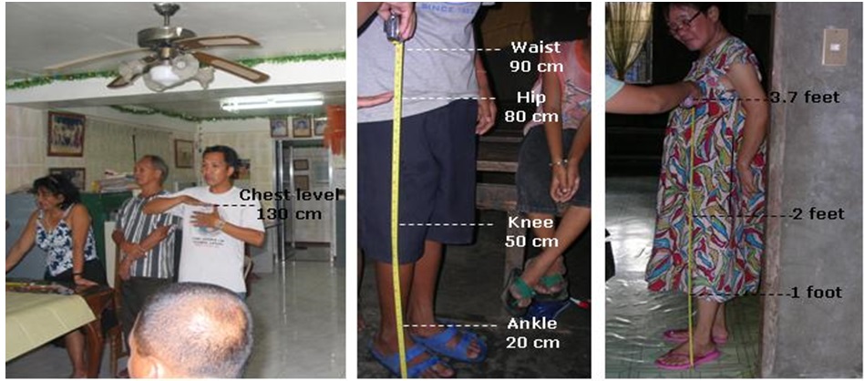
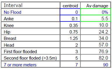
During the PGIS Survey the flood height of historical events was not recorded in centimeters, but in the way the local people indicate it. The table below shows the ‘reference' levels found during several fieldwork activities as used by the people to indicate and refer to floodwater depths. As discussed during the workshops the average of 10 cm difference in height between men and women may determine differences in the perception of hazard. In order to minimize the inconvenience this could cause the participants agreed and expressed the water depths in ranges, rather than in absolute or sharp values.

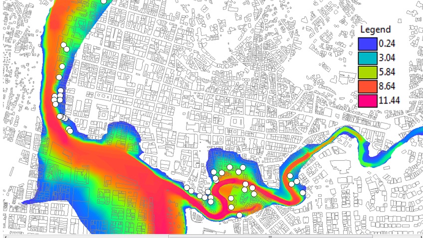
The map shows the location of the Participatory GIS survey points in relation to the flooded areas and the building footprints. The table gives an impression of the data that was collected:

 

---

Analysis steps:

Step 1: Analyzing the data collected from the field.

After a flood event, a survey was carried out in an area, and with the help opf local communities. Data from the survey contains information on:

• Building types
• Occupancy type 
• Number of floors
• Flood depth
• Flood damage

The table is linked to the point map PGIS_Location that represents the position of each interview. It is important to check the position of the interviews in relation to the flood extent; show the survey location together with the 100 years return period flood map (See above).

We can now start to work at the extraction of the depth-damage functions. The damage data stored in the table are related to the major flood occurred, the depth-damage curves will be calculated on the basis of those data. The data from the PGIS_Survey table are copied to Excel. Only the record related to floods are requested.

Step 2: Calculate the stage damage function for all buildings

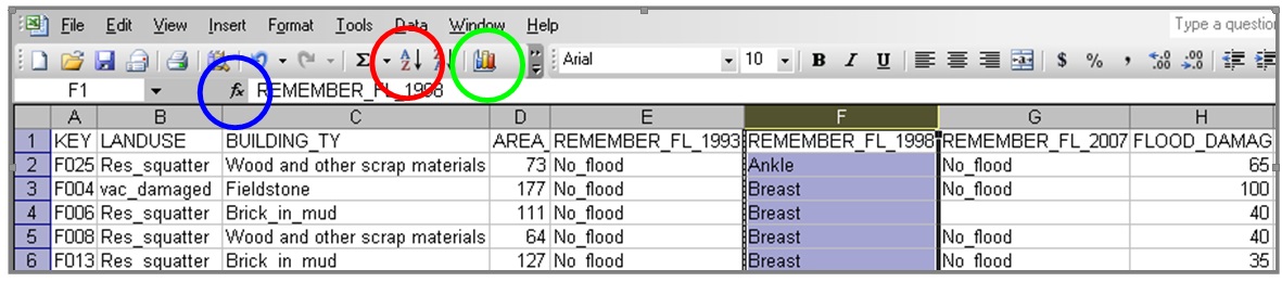
To calculate the depth-damage curves we use the records of the damages caused to the affected buildings; the data are stored in the table you just extracted in the column "Flood_damage" . This column shows the damage of the flood. We need to calculate the average of damage for each water-height interval. Sort the records by water height related to the 1998 flood event in Excel: select the right column and click the button with the red circle in figure above.  Calculate the average of damage for each water height interval. Click the "Function"  (blue circle in figure above  and chose "average" .

Build in Excel a table with at least the last two columns; it will be used to show the results in an X/Y graphic. Add a row on top and a row at the bottom as shown here below. The first line represents the situation in which the buildings are not flooded; the last line represents the extreme situation with more than 7 meters of flood depth; we can assume that, when the flood depth is 7 meters or more, the average damage for all the building types is 90% (it has been previously calculated through other methods).

Now we have to build a graph in Excel using the values of the centroid of each interval as X value and the average of the damage as Y value. Open the "Graphics menu"  in Excel by clicking the icon with the green circle in figure x.x. Chose "XY Scatter"  and click next; then go to "series"  tab; add a new series and fill the right side of the window as follows  

 

1. Select the X Values and chose the cell where you stored the centroid of the interval "Ankle"  and the cell above (blue cells in the table).
2. Select the Y Values and chose the cell where you stored the average of damages for that interval and the cell above (green cells in the table).

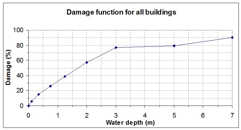
Follow the procedure for all the intervals (from "Ankle"  to "7m or more" ) and display the graphic. If you don't see the line, right-click on each pair of points, chose "format data series" , and, in "patterns"  add the line.  It should be similar to this figure.

The next step consists of fitting the trend line for each series. Right-click on each pair of points, and chose "add trend line" . In the "Type menu"  chose "linear function"  and in the "Option menu"  select "display equation on chart"  (for the "Ankle"  series select also "Set intercept = 0") .

Follow the procedure for all the series and at the end you should have the rend lines for all the points and their equations like in the following figure

Results:

All the buildings are considered with the same characteristics and the different numbers of floors are not taken into account. A single storey squatter does not have the same damage rate of a 4 storey reinforced concrete building. In order to improve the procedure we should chose a smaller aggregation level. For instance we can start to calculate the depth-damage functions only for the Landuse Residential Squatters. The following instructions show briefly the procedure to calculate the functions for squatters, if you have time and you are interested in it, try to reach the task.

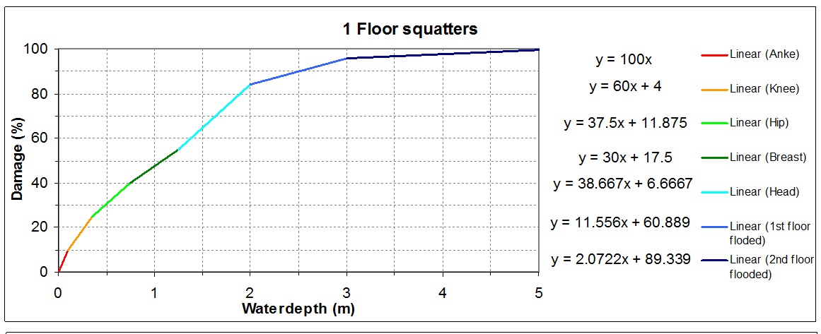
The graph is steeper than the other and it reaches values close to 80% of damage at a water depth of 2m. This is due to the higher vulnerability of the squatters that the overall average. The interval between 0.75m and 1.25 shows strange results: the squatters seem to have lower damage rates with this water depth than the average of the building types. This inconsistency is caused by the small amount of records that the statistics are based on.

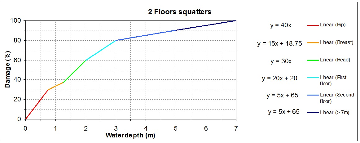
Also graphs are made for squatters with two floors

  

Conclusions:

This use case shows a method to generate vulnerability curves from damage data that has been collected using a community-based survey, and with participatory GIS. The use of local knowledge from communities is a powerful tool for managing risk at local and municipal level. The accumulated knowledge and perceptions of communities 'at-risk' are recognized as key elements in ameliorating or managing disaster risk at local level, particularly in places where much of the crucial information as well as the technical and economic resources for risk assessments are not otherwise available. 

Regarding Disasters identifying risk factors and understanding the way in which communities cope and adapt themselves to hazardous environments are considered important determinants for risk reduction and decision-making at local and municipal level.

The understanding of mechanism for coping and adaptation to flooding and other natural phenomena is not always straightforward to external actors such as researchers and policy-makers. Risk, and therefore the mechanism to deal or avoid it are perceived differently by those that see flooding as a phenomenon to measure and model, those that for instance take decisions about urban development, public investment or land use change and those who have to deal with flooding effects in their everyday life and who in consequence have to face and manage the threat.

Local knowledge can improve the way in which internal and external actors understand flood risk and take decisions about risk management and urban planning. Local people may know 'facts' not just about natural events, but also about the changes in their physical and socioeconomic situation, which lead to variations of flood risk over time. Furthermore local people behave and develop mechanisms for coping that can guide local authorities in the development of adequate measures that help at risk communities to avoid or decrease their vulnerability. 

In the last decade several tools that look for enhancing the inclusion of at risk communities coping capacities and their risk related knowledge into the decision-making process are under exploration. Methods of participatory research, such as Participatory Rural Appraisal (PRA), Rapid Rural Appraisal (RRA), and Participatory Action Research (PAR) that were initially developed to analyze local knowledge and life conditions in fields such as anthropology, and natural resource management (Gilbert et al., 1980; Scoones and Thompson, 1994; Lawas, 1997; Gonzales, 2000;Sedogo, 2002; McCall, 2003), are proven their efficiency also in local risk assessment (Ireland, 2001; Bassolé et al, 2001; UNCRD, 2003; Dekens, 2007). 

Local disaster management committees could be involved in carrying out surveys to collect relevant data for hazard and risk assessment, which includes mapping and characterization of buildings, people, livelihoods etc., identifying aspects of vulnerability and coping capacity. Also they could be involved in carrying out damage surveys after the occurrence of flood events in order to develop vulnerability curves that are suitable for the local conditions. Information on vulnerability curves should also be shared among the various countries in the Caribbean.

References:

Bassolé, A., Brunner, J., Tunstall, D. (2001). GIS: supporting environmental planning and management in West Africa. A report of the joint USAID/World Resources Institute Information Group for Africa.

Dutta, D., Herath, S. and Musiake, K., 2003. A mathematical model for flood loss estimation. Journal of Hydrology, 277(1-2): 24-49.

Gilbert, E. H., Norman, D.W, and Winch, F.E. (1980). Farming System Research: A Critical Appraisal. In MSU Rural Development Paper, Vol. 6. (East Lansing, Michigan State University).

Gonzales, R. (2000). Platforms and Terraces. Bridging participation and GIS in joint-learning for watershed management with the Ifugaos of the Philippines. PhD Thesis. ITC Dissertation No. 72. Wagenigen University.

Ireland, D. (2001). Disaster Risk Management from a Remote Shire's Perspective. Centre for DisastersStudies, JCU. Australia. 57 p.
Krzysztofowicz, R. and Davis, D.R., 1983a. Category-Unit Loss Functions for Flood Forecast-Response System Evaluation. WATER RESOURCES RESEARCH, 19(6): 1476-1480.

Krzysztofowicz, R. and Davis, D.R., 1983b. A Methodology for Evaluation of Flood Forecast-Response Systems 1. WATER RESOURCES RESEARCH, 19(6): 1476.

Lawas, C. (1997). The resource users' knowledge, the neglected input in land resource management. PhD.dissertation, ITC- Wageningen University.

Peters Guarin, G. ( 2008 ). Integrating local knowledge into GIS-based flood risk assessment. The case of Triangula and Mabolo communities in Naga City - The Philippines. ITC PhD thesis. https://www.itc.nl/library/papers_2008/phd/peters.pdf

Scoones, I., and Thompson, J. (1994). Knowledge, power and agriculture: towards a theoretical understanding. In Beyond farmer first: rural people's Knowledge, agricultural research and extension practice. (Ed) I. Scoones, and J., Thompson. Intermediate Technology.

Sedogo, L.G. (2002). Integration of local participatory and regional planning for resources management using remote sensing and GIS. Wageningen University, 2002. ITC Dissertation 92, 177 p.

United Nations Centre for Regional Development (UNCRD) (2003). Sustainability in Grass-Roots Initiatives Focus on Community Based Disaster Management. 103 pp.

United Nations International Strategy for Disaster Risk Reduction (UNISDR). (2005). Hyogo Framework for 2005-2015: Building the Resilience of Nations and Communities to Disasters. [on line 22 June 2005]. http://www.unisdr.org/wcdr/intergover/official-doc/L-docs/Hyogo-framewor....

United Nations-International Strategy for Disaster Reduction (UN-ISDR) (2002). Living with risk. A global review of disasters reduction initiatives. Geneva. Switzerland. 387 pp.

Last update: 01 - 01 - 2015