Author: Michiel Damen
One of the defining features of geoinformation science is its ability to combine spatially referenced data. A frequently occurring issue is the need to combine spatial data from different sources that use different spatial reference systems.
Most of the theory described in this chapter is derived from the ITC textbook on GI Science and Earth Observation, Chapter 3. Click here to download the textbook.
Reference surfaces
The surface of the Earth is far from uniform. Its oceans can be treated as reasonably uniform, but the surface or topography of its land masses exhibits large vertical variations between mountains and valleys. These variations make it impossible to approximate the shape of the Earth with any reasonably simple mathematical model.
Consequently, two main reference surfaces have been established to approximate the shape of the Earth : one is called the Geoid , the other the ellipsoid. See figure 1.
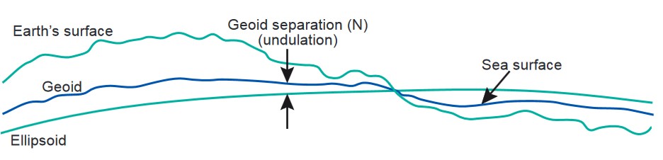
Figure 1. The Earth's surface and two reference surfaces used to approximate it: the Geoid; and a reference ellipsoid. The Geoid separation (N) is the deviation between the Geoid and the reference ellipsoid.
The Geoid and the vertical datum
We can simplify matters by imagining that the entire Earth's surface is covered by water. If we ignore effects of tides and currents on this global ocean, the resultant water surface is affected only by gravity. This has an effect on the shape of this surface because the direction of gravity" ”more commonly known as the plumb line" ”is de plumb line pendent on the distribution of mass inside the Earth. Owing to irregularities or mass anomalies in this distribution, the surface of the global ocean would be undulating. The resulting surface is called the Geoid (Figure 2). A plumb line through any surface point would always be perpendicular to the surface.
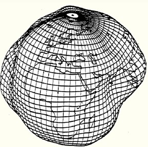
Figure 2. The Geoid, exaggerated to illustrate the complexity of its surface.
In order to establish the Geoid as a reference for heights, the ocean's water level is registered at coastal locations over several years using tide gauges. Averaging the registrations largely eliminates variations in sea level over time. The resultant water level represents an approximation to the Geoid and is termed mean sea level.
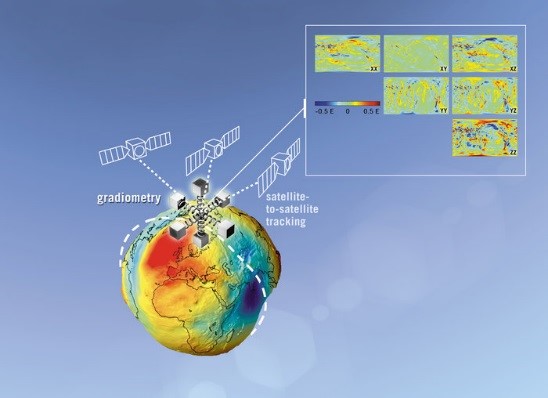
Figure 3. The GOCE mission of the European Space Agency (ESA) takes six simultaneous measurements of the gravity field.
Several definitions of local mean sea levels (also called local vertical datums) appear throughout the world. They are parallel to the Geoid but offset by up to a couple of metres to allow for local phenomena such as ocean currents, tides, coastal winds, water temperature and salinity at the location of the tide gauge. Care must be taken when using heights from another local vertical datum. This might be the case, for example, in areas along the border of adjacent nations. Even within a country, heights may differ depending on the location of the tide gauge to which mean sea level is related. As an example, the mean sea level from the Atlantic to the Pacific coast of the U.S.A. differs by 0.6" “0.7 m. The local vertical datum is implemented through a levelling network, which consists of benchmarks whose height above mean sea level has been determined through geodetic levelling. As a result of satellite gravity missions, it is currently possible to determine height above the Geoid to centimetre levels of accuracy.
For the website of Gravity mission GOCE of the ESA, click here.
The Ellipsoid
The Geoid is a as a reference surface for heights. We also need, however, a reference surface for the description of the horizontal coordinates of points of interest. To project these horizontal coordinates onto a mapping plane, the reference surface for horizontal coordinates requires a mathematical definition and description. The most convenient geometric reference is an ellipsoid. It provides a relative simple figure that fits the Geoid to a first-order approximation. In geodetic practice is the ellipsoid defined by its semi-major axis and flattening f. See figure 4.
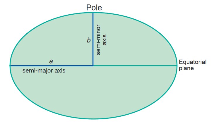
Figure 4. Ellipsoid defines by its semi-major axis a. and semi-minor axis b.
Flattening f. is dependent on the semi-major and semi-minor axes. f = (a " “ b) / a.
An example of typical values are: a: 6378135.0 m; b: 6356750.52 m. There exist various ellipsoid models; WGS84 is a global standard for many satellite coordinate reference systems. See also figure 5.
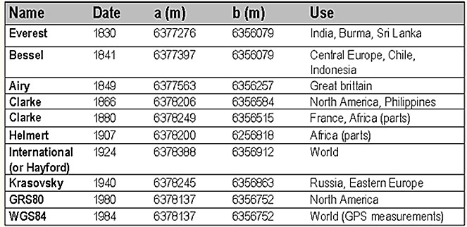
Figure 5. Examples of ellipsoid a. and b. values. WGS84 is a global standard reference system
Because of different topographies per region, there exist also differences in height above the Ellipsoid (h) and Geoid (H). In particular with the use of Digital Elevation Models it is crucial to select the correct ellipsoid values, or Datum in the Geographic Information system to be used.
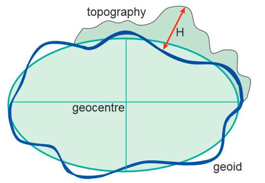
Figure 6. Height of topography above ellipsoid (h) and geoid (H)
Map Projections
By definition, any map projection is associated with scale distortions. There is simply no way to scale distortions flatten an ellipsoidal or spherical surface without stretching some parts of the surface more than others. The amount and kind of distortions a map has depends on the type of map projection.
There exist basically three classes of projections; these are Cylindrical, Conical and Azimuthal. The azimuthal, conical, and cylindrical surfaces in Figure 7 are all Tangent surfaces, i.e. they touch the horizontal reference surface at one point (azimuthal), or along a closed line (cone and cylinder), only. Another class of projections is obtained if the surfaces are chosen to be Secant to (to intersect with) the horizontal reference surface (Figure 8). Transverse Cylindrical and Oblique Conical projections are projections where the reference surfaces are not horizontal but tilted (Figure 9).
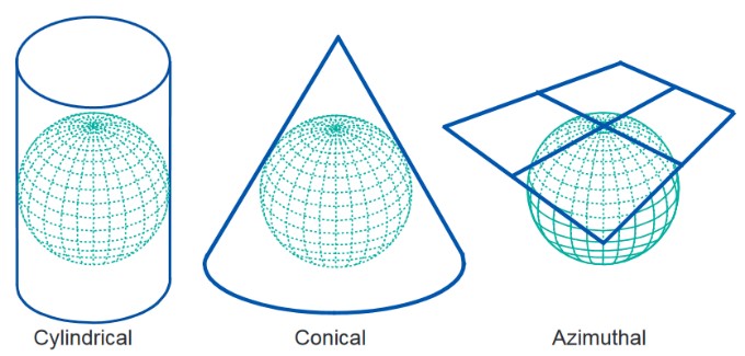
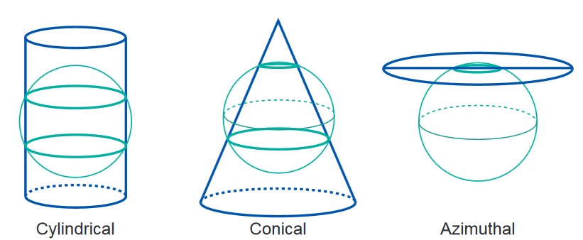
Figure 7 (LEFT) Basic types of tangent map projections
Figure 8 (RIGHT) Basic types of secant map projections.
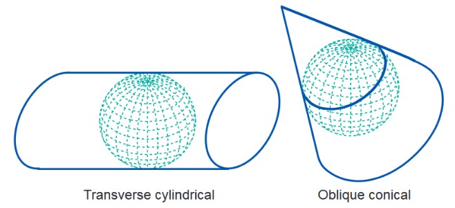
Figure 9. Transverse cylindrical and Oblique conical projections.
The Universal Transverse Mercator (UTM) is a system of map projection that is used worldwide. It is derived from the Transverse Mercator projection (also known as Gauss-Kruger or Gauss conformal projection). UTM uses a transverse cylinder secant to the horizontal reference surface. It divides the world into 60 narrow longitudinal zones of 6 degrees, numbered from 1 to 60. The narrow zones of 6 degrees (and the secant map surface) make the distortions small enough for large-scale topographic mapping.
So far, we have not specified how the curved horizontal reference surface is projected onto a plane, cone or cylinder. How this is done determines what kind of distortions the map will have compared to the original curved reference surface. The distortion properties of a map are typically classified according to what is not distorted on the distortion properties map:
With a conformal map projection, the angles between lines in the map are identical to the angles between the original lines on the curved reference surface. This means that angles (with short sides) and shapes (of small areas) are shown correctly on the map.
With an equal-area (equivalent) map projection, the areas in the map are identical to the areas on the curved reference surface (taking into account the map scale), which means that areas are represented correctly on the map.
With an equidistant map projection, the length of particular lines in the map are the same as the length of the original lines on the curved reference surface (taking into account the map scale)
Map Projections in the West Indies
Most of the maps and data used in the West Indies apply a conformal projection using a horizontal/longitudinal cylinder. This projection is referred to as Transverse Mercator, and is specific for the given areas. In order to reduce the problems associated with cross country unique projections and datums, cartographers and geomatics scientists use the internationally most used Universal Transverse Mercator (UTM) projection.
To transform data from one type to another, certain parameters are required. The most common transformations used in the Caribbean are the 3-parameter geocentric translation shifts; the 7-parameter Helmert transformation and the 10-parameter Molodensky transformation. The geocentric translation is a simple 3-dimentional shift in the X,Y,Z axes assuming that projected lines are exactly parallel and that there are no scale differences. However, the other transformations model has non-parallel projective differences and has scale distortions in addition to the translational shifts. Unlike the 3-parameter solution, the 7-parameter solution requires many highly accurately collated points to compute; contributing to the lack of good transformation parameters in the Caribbean. Table 1 shows common datums and projections in the Caribbean.
Table 1 : Common Datums and Projections in the Caribbean
|
Country |
Projection |
Datum |
Shifts |
Scaling |
Coordinates of Origin |
False Origin |
|---|---|---|---|---|---|---|
|
St. Vincent (Mugnier, 2004a) |
BWI Transverse Mercator Grid |
St. Vincent Datum of 1946 based on the Clarke 1880 |
St. Vincent Datum of 1946 to WGS 84 ∆X = +196 m ∆Y = +332 m ∆Z = +275 m |
0.9995 |
Central Meridian = 62º W latitude of origin = equator |
E =400,000m |
|
St. Lucia (Mugnier, 2004b) |
BWI Transverse Mercator Grid |
St. Lucia Datum of 1955 based on the Clarke 1880 |
St. Lucia Lighthouse 1955 Datum to the WGS 84 ∆X = " “134 m ∆Y = +119 m ∆Z = +314 m |
0.9995 |
Central Meridian = 62º W latitude of origin = equator |
E =400,000m |
|
St. Lucia (Fugro 2009) |
BWI Transverse Mercator Grid |
St. Lucia Datum of 1955 based on the Clarke RGS |
St. Lucia 1955 Datum to the WGS 84 ∆X = " “149 m ∆Y = +128 m ∆Z = +296 m |
0.9995 |
Central Meridian = 62º W latitude of origin = equator |
E =400,000m |
|
Grenada (Mugnier, 2005) |
BWI Transverse Mercator Grid |
Grenada National Grid of 1953 based on the Clarke 1880 |
Grenada 1953 Datum to WGS 84 ∆X = +72 m ∆Y = +213 m ∆Z = +93 m |
0.9995 |
Central Meridian = 62º W latitude of origin = equator |
E =400,000m |
|
Dominica (ESRI) |
BWI Transverse Mercator Grid |
Dominica National Grid of 1945 based on the Clarke 1880 ellipsoid |
Dominica 1945 datum to WGS 84 ∆X = +725 m ∆Y = +685 m ∆X = +536 m |
0.9995 |
Central Meridian = 62º W latitude of origin = equator |
E =400,000m |
|
Dominica (JICA) |
BWI Transverse Mercator Grid |
Dominica National Grid of 1945 based on the Clarke 1880 ellipsoid |
Dominica 1945 datum to WGS 84 ∆X = +? m ∆Y = +? m ∆X = +? m |
0.9995 |
Central Meridian = 62º W latitude of origin = equator |
E =400,000m |
|
Belize (Mugnier, 2009) |
Transverse Mercator Grid NAD 27 |
NAD27 To WGS84 ΔX = 0 m ±8 m ΔY = +125 m ±3 m ΔZ = +194 m ±5 m |