2.2 Flood data

Flood models (like LISEM) use input data directly to determine the hydrological processes that it simulates. This information is broken down into hydrological variables related to interception of rainfall and resistance to flow.  The user has to break these classes down into hydrological variables for cover, infiltration related parameters and surface flow resistance.

Nevertheless in this project a PCRaster script is made to create the 5 data groups for a model run (columns in figure 1), for which basic maps are needed (row 1). Using a combination of field data and literature (row 2) the input database for the model is created (row 3). Table 1 describes briefly the main base maps, their origin if known, and how they are used in LISEM. 

Figure 1. Flow chart of the creation of an input database for LISEM from 5 basic data layers. The database is generated automatically in a GIS (PCRaster) with a script that is tailor made for a country. 

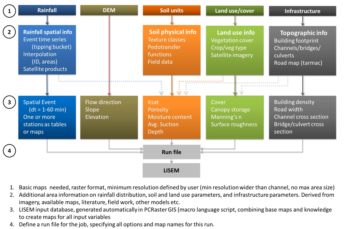
Table 1. List of main data layers as example for St Lucia and their origin and main GIS operations

 

DEM and derivatives

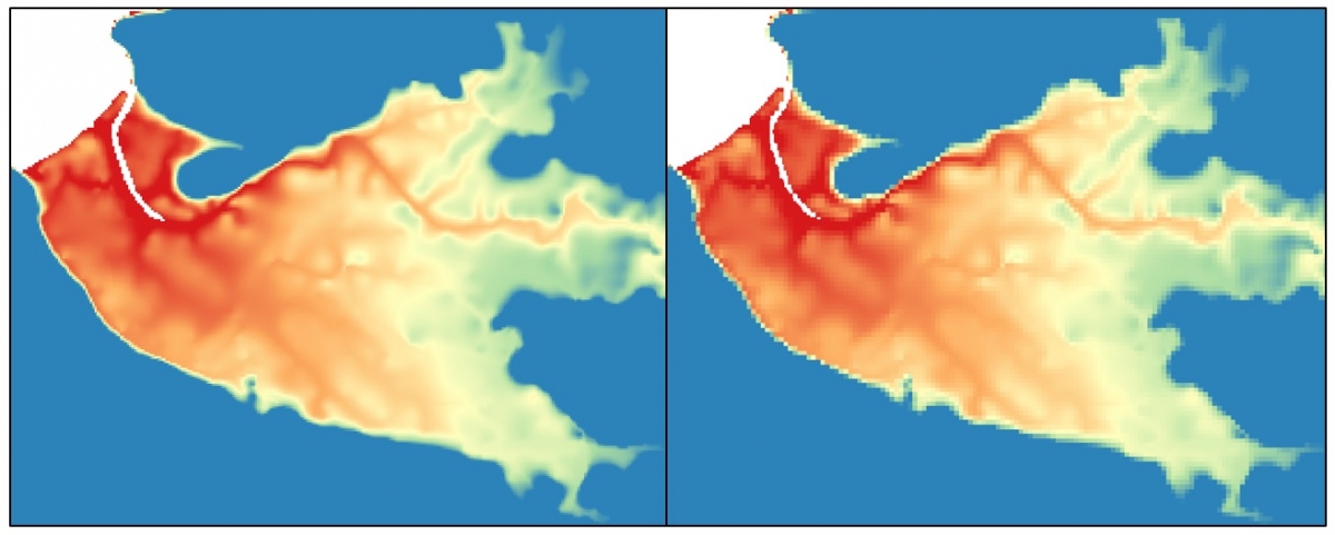
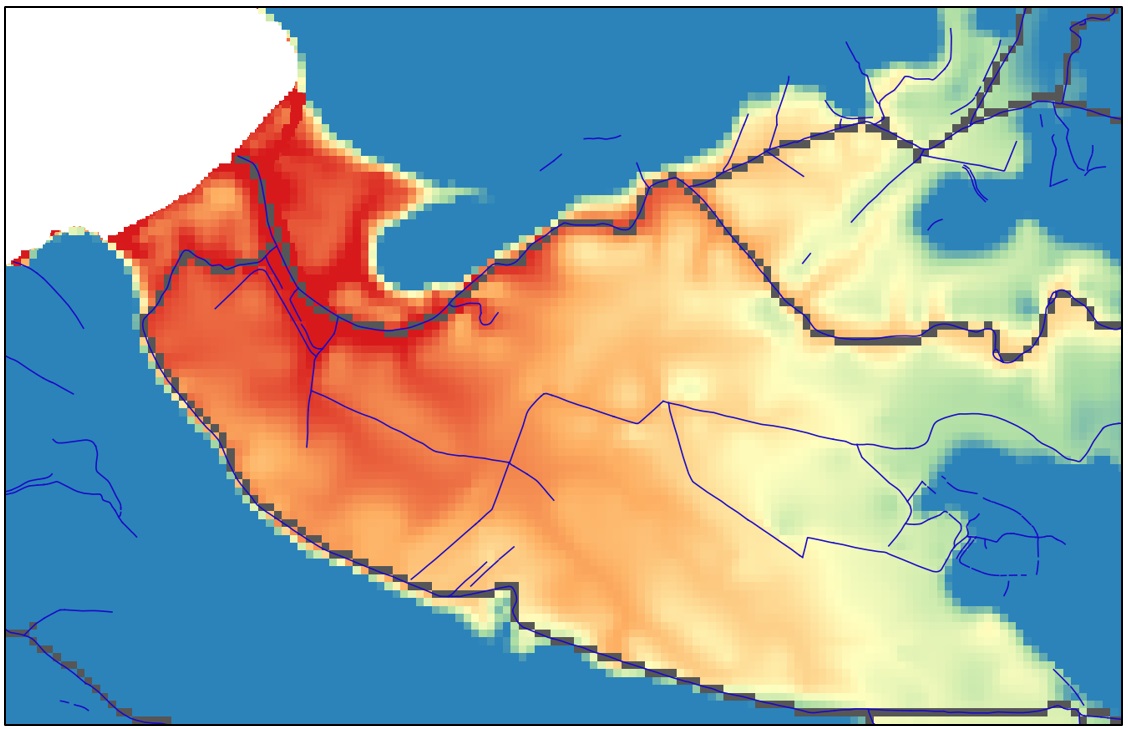
The DEM is used for overland flow directions and slope in the runoff part of the model, and the elevation is used directly in flood modelling. The DEM of St Lucia is created by a Kriging interpolation from elevations lines using an exponential semivariogram. The elevation contours have 2m spacing, and the interpolated map was produced on a 10m resolution. This was then resampled to a 20m resolution using the average of 2x2 cells. It is not known what the origin of the contour lines is. They seem to be generated automatically from another source but the meta data is not available. Nevertheless they do contain some detail in the flood plain as can be seen in figure 2. The resampling did not significantly change the level of detail.

The absolute accuracy of the DEM is not known, but a good check is if the digitized river (derived from air photos or images), follow the DEM depressions (see below). This is an indication that the natural depressions and small variations in the flood plain, with elevation details of less than 0.5 m, are faithfully reproduced. 

Figure 2. DEM in 10m resolution (left) and 20m resolution (right) based on Kriging of the elevation lines. The area shown is Roseau river floodplain and bay on St Lucia. The elevation scale is scaled from 0 (red) to 10m (blue) to show the detail in the flood plain. The section shown is 3750m in width.

Soil depth

The soil depth is unknown and in spite of the simplicity of the parameter, it is not well studied and few algorithms exist to generate a soil depth map. Kuriakose et al., (2009) generated soil depth for a mountainous catchment in the southern India, in the Ghats Mountains. The research was part of a landslide research where soil depth was one of the more important parameters. The situation is very similar to the Caribbean islands: tropical wet climate (Monsoon driven), soil formation due to weathering, although not from volcanic origin, and rapid denudation that causes slopes with thin soils and valleys that are filled up with debris over time, by erosion and mass movement. Derived from this research, the following GIS operation was used to create a soil depth map (in m):

Soil depth = a((1-S) -  b D_river + c D_sea^d)^e

 where:S = terrain slope (bounded 0-1)

D_river = is the relative distance to the river channel (0-1)

D_sea = the relative distance to the sea (0-1)

Scaling parameters: a=1.5, b=0.5, c=0.5, d=0.1, e=1.5

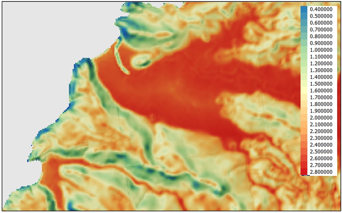
The logic is that steeper slopes have shallower soil, closer to the river the soil depth increases, and closer to the sea the soil depth decreases. Visual field checks have been limited to observations of river depth (surface to bedrock) along Bois d'Orange river, Choc river, Roseau river and the rivers near Dennery and Castries. Figure 3 shows the soil depth for the areas shown above. The river depth is simply the soil depth in the channel pixels.

Figure 3. Example of soil depth (in m) generated from the DEM, river system and proximity to the sea. 

River network and river dimensions

A shape file with drainage lines exists in the St Lucia database, classified as artificial (small drains along the roads) and natural channels. The latter class, the natural channels, have been used in the flood model, because at the national scale drainage along roads cannot be modelled. However, the hydrological quality of the digitized map is not very high, almost all river sections are digitized separately and there is no connectivity, so the river network shape file does not constitute a continuous flow network. Also under vegetation the rivers are not easy to spot and are sometimes not visible at all. This also leads to network fragments, and moreover these flow lines are not always in the deepest part of the valleys. It is impossible to use this network directly in the model (or any model) as flood water that overflows will flow into the deepest points of the valley and cannot drain from there. The simulated flood hazard would be more severe than it is in reality.

In contrast in the flat coastal plains and river mouths, the DEM does not have enough information to generate a valid flow network, but there the rivers can be well seen on high resolution imagery and the digitized river networks are of a higher quality.

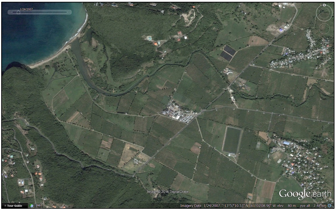
The final river network was created by combining the visible coastal plain sections with an automatically generated river network based on the DEM for the upstream areas. There is no automatic procedure for this. All rivers were corrected and checked by hand, and a river channel mask map was produced on a 10m and a 20m resolution. Figure 4 shows a comparison of Roseau bay. The man made channels are not included in the national flood hazard map, as their dimensions are very small.  

Figure 4. Stream network example of Roseau bay, with a high res image (24 Jan 2007) from Google Earth  (top) and the digitized stream network (blue lines) and 20m raster river network used in the flood model (dark grey).

From the river network at 20m, the channel dimensions are derived automatically. It is assumed that the river dimensions increase from the source to the outlet near the see. Note that LISEM has the restriction that the river channel cannot be wider than the gridcell, because the flow is a 1D kinematic wave in the converging channel network. The algorithm used is based on Allen and Pavelski (2015) who show that for large North American river systems there is a good correlation between total rive length and river width. They further extrapolated their data to smaller river systems, using the total river surface area, and correlated that to river width (r² = 0.996, p < 0.001):

                Area = 3.22e4 * W^-1.18

This equation is used in the dataset, whereby the river area is approximated as the accumulation of cell area from the river source to the outlet. Fig 5.5show the effect for the Roseau river mouth.

Figure 5. Example of the river width algorithm near L'Anse la Raye. The river mouth is wider than results from the algorithm but the river sizes several 100m form the coast line are close (between 6 and 7 m in the top red circle and 9 and 10m in the bottom red circle). 

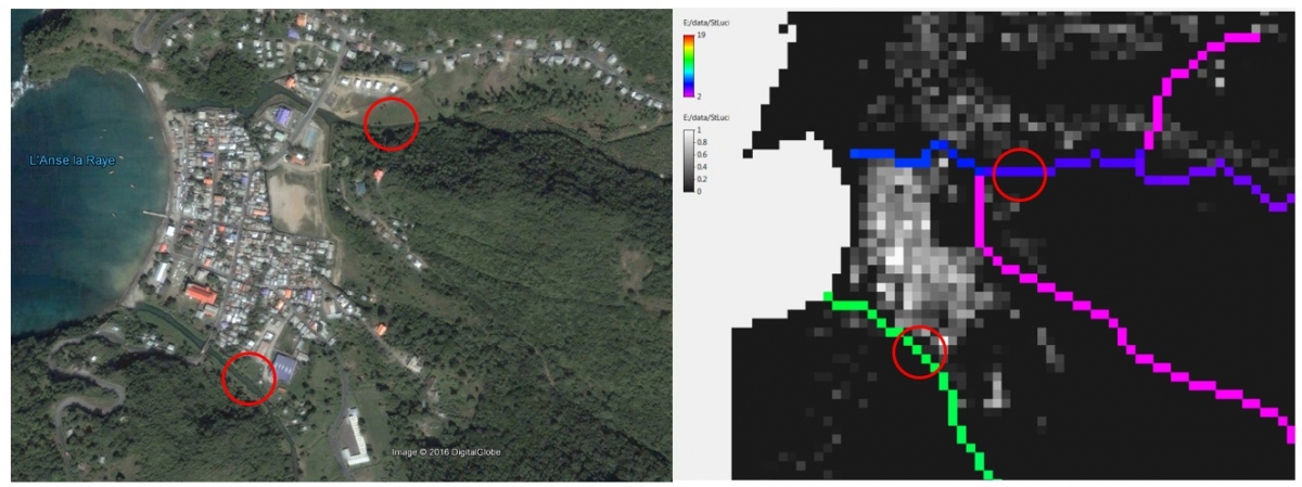
Everywhere it is observed that the river has eroded until bedrock, apart from the last kilometer or so near the mouth, where sedimentation takes place and the river widens. This river depth was estimated by using the soil depth as river depth. The soil depth is generated from the DEM as explained below.

Important: at the national scale sedimentation of sand and debris in the river beds is not included. Occasionally this may cause obstruction of culverts and bridges, or greatly decrease the storage capacity of the channels. Hence the flood map shows the situation with clear rivers with maximum capacity, using the assumptions of dimensions as explained above.

The river network in LISEM is characterized by two more parameters: the slope of the river bed and the resistance to flow (Manning's n). The slope of the river bed is obtained by taking the slope of the DEM in its steepest downstream direction. The Manning's n is taken from comparing observations in the field with literature values. Morgan et al. (1998) has compiled a large number of values for different surfaces, and the USGS websites provides visual references: http://www.rcamnl.wr.usgs.gov/sws/fieldmethods/Indirects/nvalues/. Generally the riverbeds are either sedimented or rocky with boulders which gives a Manning's n of 0.03-0.04, and the banks are overgrown with abundant natural vegetation, so the value was increased to 0.05. 

Soil map and derivatives

The island is of volcanic origin with an active volcanic site comprising near surface hydrothermal hot spots with geothermal energy potential. St. Lucia can be described as geologically young not exceeding 50 million years with rocks such as rhyolite, andesite and various basalts (Towle et al, 1991, in WRMU, 2001). The rock formations present are classified into three series:

• Northern Series (Early Tertiary- Eocene) -  older rocks predominantly basaltic in composition, heavily folded and of Eocene age. In some areas in the north one can find Andesite Porphyry and Rhyolite.
• Central Series (Middle Tertiary -  Miocene / Pliocene) -  the central ridge (Barre D'Iisle) and the rocks underlying the eastern coast were formed thirty to forty million years ago due to an extended sequence of volcanic activity which generated extrusions of younger andesite, basalts, agglomerates and tuffs.
• Southern Series (Mid to Late Pleistocene)- the southern region in the area of the pitons, the volcano as well as Mount Gimie (the highest peak) can be found the newest (geologically) dacite segment. The region near the volcanic crater evolved when there was volcanic activity with dacite and pyroclastics after a series of thirty-three consecutive eruptions, which triggered avalanches of andesite pumice on the adjacent slopes

The soils that came into existence from this volcanic parent are generally fertile and rich in clay and silt. The valley floors are generally filled with material form erosion and mass movement from the slopes, and can be more sandy in nature because of the lateral sorting process, where clay in suspension is washed out. Near the coast the material is also more sandy. All soils are gravelly to some degree, the gravel resulting from weathering processes of the parent material.

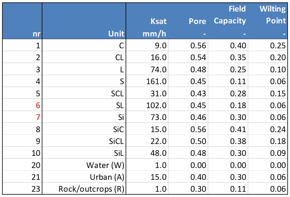
The soil map originates from 1966 soil map made by UWI Imperial College of Tropical Agriculture. The soil Classification system is general for the islands, designed by the authors (Stark et al., 1966)) of these maps. It is important to note that the soil mapping was primarily based on topography, drainage, parent material and not according to pedology which emphasizes how the soils originated. The approach taken by the surveyors reflected the need to produce a survey that would be of most use for the agricultural community, not for its potential use in geotechnical investigations (CDERA, 2006). The classification system follows the US convention of assigning a "typical soil profile" and giving them a name based on the type location, such as "Anse Clay" or "Mabouya Silty Clay". Each of these units have a texture class indication according to the USDA texture class triangle, and the class average grain size distribution was assumed. Based on the texture class the soil physical parameters Saturated Hydraulic Conductivity (Ksat in mm/h), Porosity (cm³/cm³) and average initial matric suction (kPa) were derived, using the pedotransfer functions of Saxton and Rawls (1986), see figure 6). This results in the values in table 2. The pedotransfer functions are largely texture based, with effect of stoniness and organic matter. The stoniness is information given for each soil class in the soil map which causes a small effect on Ksat and somewhat larger on porosity (Saxton and Rawls, 1986):

Ksat_eff = Ksat*(1 - stone)/(1 -  0.85*stone)

Pore_eff = Pore*(1-stone)

It is known however that the soil structure has a large effect on the Ksat and porosity. Normally a soil classification system is not based on the top soil as this is often affected by agriculture and building activities. The texture indications are valid for both top soil and subsoil, but under natural vegetation the top soil has a much more open structure. The clayey soils, derived from weathered volcanic material, form strong and stable aggregates under natural conditions, that give the soil an open structure with a high porosity and high saturated hydraulic conductivity. This means that the top soil can absorb quickly large amounts of water, depending on how dry it is. Under agricultural circumstances the tops soil is more massive during most of the year, for instance as in the frequently occurring Banana plantations. Trampling of the soil destroys its structure.

Figure 6. Pedotansfer functions by Saxton and Rawls (1986) used in SPAW model software.

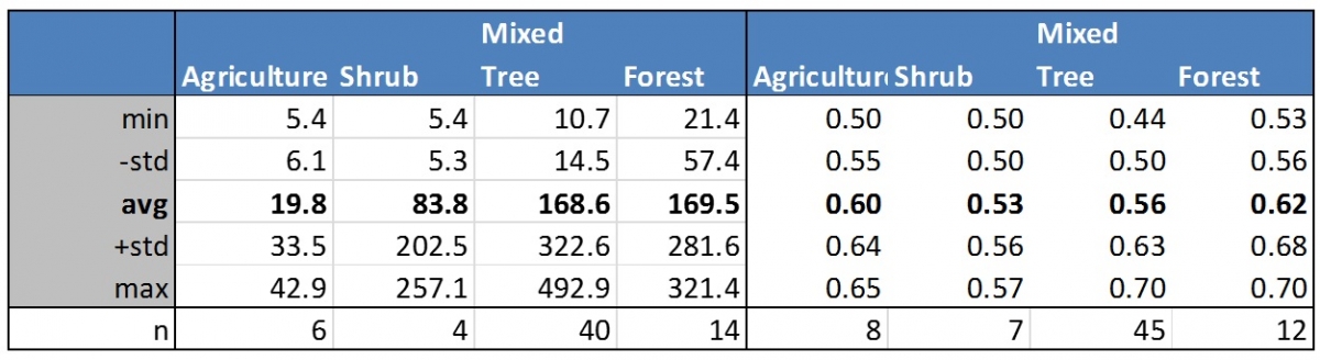
As is common in tropical environments, the organic matter rapidly decreases with depth because of the high degree of decomposition. This was confirmed by Pratomo (2015) who determined the saturated hydraulic conductivity from 64 sample rings and porosity from 72 sample rings on Grenada, in the Gouyave and St John watersheds as part of a comparative catchment study in the CHARIM project. It is clear from figure 7 and table 2, that the ksat under natural vegetation is a lot higher than the statistical values for the clays and silty clays in the area (table 3). This is attributed to the high organic matter content and open structure of the forest soils. The agricultural area was clearly closer to the statistical values found by Saxton and Rawls (1998), although there is a large spread as is also common for conductivity. The porosity values are generally high which is also common to clay rich soils and there is much less variation.

Figure 7. Left: saturated hydraulic conductivity (mm/h) and right: porosity (-) organized per main land cover type. The measurements are from Grenada, taken in the Gouyave and St John watersheds (Pratomo, 2015). The values in bold are the average, the lines show one standard deviation around the mean.

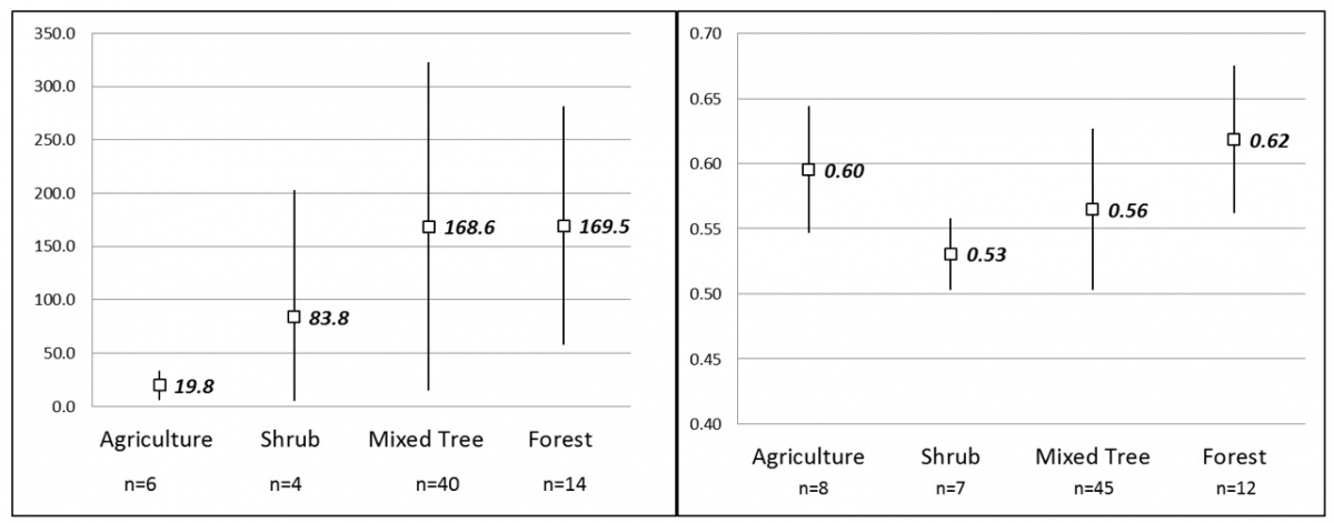
Table 2. Basic statistics of soil physical parameters measured in Grenada in the Gouyave and St John catchments, in clays and silty clays (Pratomo, 2015).

It was therefore decided to use a two layer Green and Ampt infiltration model in LISEM, whereby the top layer of 15 cm, has larger values of Ksat and porosity than the second layer for all land cover types that consist of natural vegetation (see table 4, column 4 and 5).

The advantage of this approach is that the forested areas have a larger buffering effect than would be evident form the soil texture alone. Also land use changes have a larger effect on the hydrology and flood dynamics than if soil units are directly used, which is assumed to reflect the reality better.

Table 3. Main classes derived from the soil map and assumed saturated hydraulic conductivity (Ksat in mm/h), Porosity (pore in cm3/cm3), field capacity and wilting point (cm3/cm3), after Saxton and Rawls (1986).

The Green and Ampt infiltration process in LISEM needs the matric suction at the wetting front, based on the initial moisture content that is assumed. All simulations of the flood hazard use an initial moisture content (θi) of 0.75 of the porosity (θs), which is approximately at field capacity (θfc) or slightly wetter. Since the porosity is adapted to the presence of natural vegetation, the initial moisture content is adapted as well. The matric suction (psi in kPa) is calculated directly from the initial moisture content using the following set of equations (Saxton and Rawls, 1986):

psi = a θi^-b

where:

b = (ln(1500)-ln(33))/(ln(θfc)-ln(θwp))

a = exp(ln(33)+b ln(θfc))

1500 33 = matric suction for resp. wilting point and field capacity (kPa)

 

Land cover map and hydrological parameters

A 2014 land cover map of St Lucia was created by the British Geological Survey as part of the framework of the European Space Agency (ESA) " Eoworld 2"  initiative. The following description is provided (CHARIM Data management book, section basic data collection):

" The satellite data comprised Pleiades imagery (acquired between 2013-2014) and RapidEye imagery (acquired 2010-2014). These datasets have a spatial resolution (pixel size) of 2m and 5m, respectively, for the multispectral waveband images. Additionally, the Pleiades datasets includes a very high-resolution 0.5m panchromatic image. To enable the most detailed information to be resolved, the Pleiades imagery was used as the primary dataset for generation of the new land use/land cover maps for the three AOIs; thus achieving a spatial resolution of 2m, which is equivalent to a mapping scale of 1:10,000. For each of the AOIs, land use/land cover was mapped using a combination of automated image classification, rule-based refinement and manual digitization. The existing 30m maps were used to define the different land use/land cover types and identify representative areas in the imagery to help guide the initial automated classification and to subsequently validate the mapping. Water features and the basic road networks were manually digitized at 1:10,000-scale from Pleiades imagery that had been pan-sharpened to 0.5m resolution using the panchromatic image. Wherever available, existing vector layers were utilized as baseline information during mapping.

The land use/land cover maps were validated using a standard remote sensing approach, which involves comparing the land use/land cover class identities of a sample of pixels in the map with their 'true' land use/land cover class. The 'true' land use/land cover classes of these pixels were determined using a combination of the pan-sharpened Pleiades imagery and existing maps. Consequently, the maps for St. Lucia, Grenada, and St. Vincent and the Grenadines were found to have accuracies of 84.9%, 84.8% and 80.8%, respectively; which are within the desired target accuracy of 80-90%. Additional validation of the maps for St. Lucia and Grenada was achieved using point-sampled field observations at a number of locations."

The land cover types are reclassified according to their hydrological characteristics. For event based surface hydrology only the major land cover types are important. The 2014 land cover types have therefore similar values if they are hydrologically similar (such as Evergreen forest and Semi-deciduous evergreen forest). The parameter values used in LISEM are shown in table 3.

The parameters derived from the land cover are those affecting the soil surface structure which affects infiltration, and roughness, which affects the surface runoff. Also the canopy storage for interception is derived from the land cover type. A soil cover that does not change in time is assumed, which is less realistic for agricultural areas. Cover influences the interception of rainfall by the plant canopy. This is usually in the order of 1-2 mmm (De Jong and Jetten, 2007). The variable Ksat_nat and Pore_nat (table 4) are used for the top layer Ksat and porosity under natural vegetation.

Table 4. Average vegetation parameters based on field observations.

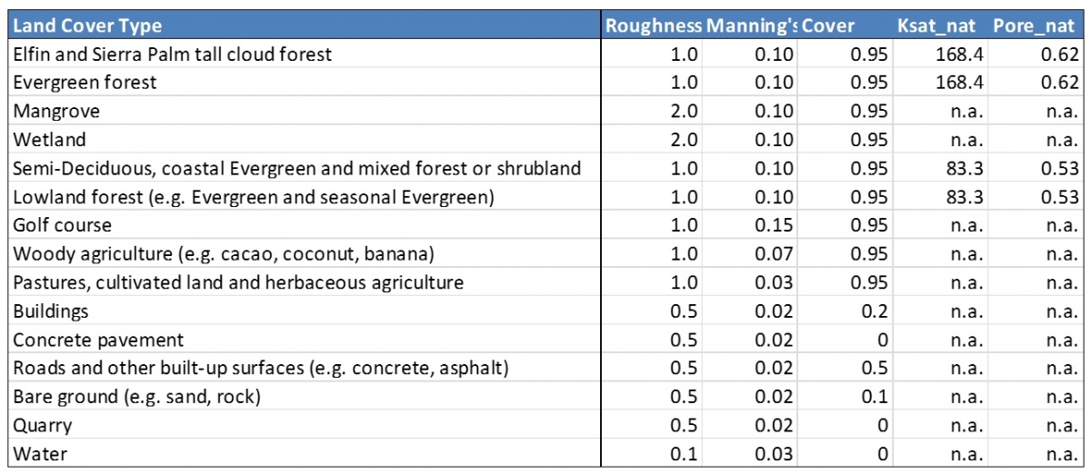
The values that are used for anthropogenic cover (built up area, concrete, roads etc) represent the value of soils adjacent to a house or road. As explained in figure 3.3, LISEM uses different layers with information on houses, roads, parking lots etc. as fractions of surface occupied, and the model needs to know the hydrological characteristics of the surface in etween these structure, or next to the road in a cell.

Building density map

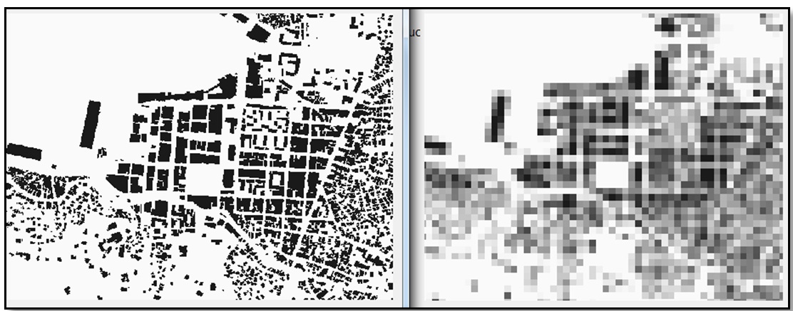
The building density map is derived from the building footprint (FUGRO, 2004) that is available in the national GIS database as a shape file. Figure 7 shows an example for the center of Castries. The building density influences the interception of rainwater, infiltration (impermeable) and the flow velocity in overland flow and floods, but the influence of individual buildings cannot be simulated at this national scale. This map is created by rasterizing the building polygons to a 2m raster, and resampling that to 20x20m to a fraction of building density per cell (0-1).

Figure 8. Rasterized building footprint at 2m resolution (left) from the center of Castries. The 20m building density (right) is used in the model.

Roads, bridges, dikes

The road shapefile has three types: 1 is the main highway, 2 are primary roads and 3 are secondary roads. All roads in the shape file are tarred roads or paved with concrete slabs. Therefore they are hydrologically smooth, impermeable and have no virtually surface ponding. The roads are reclassified to the LISEM input map according to their width. The highway is assumed to be 10m wide, the primary roads 6m wide and the secondary roads 4m wide.

Not that at the national scale, the road drainage channels are not included, as they are too small. Also the fact that at some locations the road is elevated above the flood plain like a dike, is not included, as that information is not available. 

References

Allen, G.H. and Pavelski, T.M. 2015. Patterns of river width and surface area revealed by the satellite-derived North American River Width data set. AGU Geophysical Research Letters 10.1002/2014GL062764.

Baartman, J.E.M., Jetten, V.G., Ritsema, C.J. and de Vente, J. 2012. Exploring effects of rainfall intensity and duration on soil erosion at the catchment scale using LISEM : Prado catchment, SE Spain. In: Hydrological processes, 26 (2012)7 pp. 1034-1049.

CDERA. 2006. Development of Landslide Hazard Maps for St. Lucia and Grenada. Final Project Report for the Caribbean Development Bank (CDB) and the Caribbean Disaster Emergency Response Agency (CDERA).

Chow, V.T., Maidment, D.R. and Mays, L.W. 1988. Applied Hydrology. McGraw-Hill Publishing Company; International edition. pp588.

Coles, S. 2001. An Introduction to Statistical Modeling of Extreme Values,. Springer-Verlag. ISBN 1-85233-459-2.

Cooper, V. and Opadeyi, J. 2006. Flood hazard mapping of St. Lucia. Final report for the Caribbean development bank, February, 2006.

De Jong, S. M. and V. G. Jetten 2007. "Estimating spatial patterns of rainfall interception from remotely sensed vegetation indices and spectral mixture analysis." International Journal of Geographical Information Science 21(5): 529–545.

Delestre, O., Cordier, S., Darboux, F., Mingxuan Du, James F., Laguerre, C., Lucas, C., Planchon, O. 2014. FullSWOF: A software for overland flow simulation.
Advances in Hydroinformatics - SIMHYDRO 2012 - New Frontiers of Simulation, 221-231, 2014.

Hessel, R., Jetten, V.G. and ... [et al.] 2003. Calibration of the LISEM model for a small loess plateau catchment. In: Catena, 54 (2003)1-2 pp. 235-254.

Klein Tank, A.M.G., Zwiers, F.W. and Xuebin Zhang. 2009. Guidelines on Analysis of extremes in a changing climate in support of informed decisions for adaptation. WMO Climate Data and Monitoring WCDMP-No. 72.

Kuriakose, S. L., S. Devkota, Rossiter, D. and Jetten, V.G. 2009. "Prediction of soil depth using environmental variables in an anthropogenic landscape, a case study in the Western Ghats of Kerala, India." Catena 79(1): 27-38.

Lumbroso, D.M., S. Boyce, H. Bast and N.Walmsley. 2011. The challenges of developing rainfall intensity – duration – frequency curves and national flood hazard maps for the Caribbean. The Journal of Flood Risk Management, Volume 4, Number 1, January 2011 , pp. 42-52(11).

Marmagne, J. and Fabrègue, V. 2013. Hydraulic assessment for flood risk assessment in Soufriere, Fond St Jacques and Dennery. Huricane Tomas Emergency Recovery Project, parts 1, 2 and 3. EGISeau, RIV 22852E.

Morgan, R. P. C., J. N. Quinton, et al. (1998). The European Soil Erosion Model (EUROSEM): documentation and user guide. version 3.6. SIlsoe, Bedford, UK, Silsoe College, Cranfield University: 124.

Pratomo, R.A., 2015. Flash flood behaviour on a small caribbean island: a comparison of two watersheds on grenada. MSc thesis, Applied Earth Science-Natural Hazard and Disaster Risk Management. ITC, Utrecht University, the Netherlands, pp 84.

Sánchez-Moreno, J.F., Jetten, V.G., Mannaerts, C.M. and de Pina Tavares, J. 2014. Selecting best mapping strategies for storm runoff modeling in a mountainous semi - arid area. In: Earth surface processes and landforms, 39 (2014)8 pp. 1030-1048.

Saxton, K. E., W. J. Rawls, et al. 1986. Estimating generalized soil-water characteristics from texture." Soil Sci. Soc. Am. J. 50(4): 1031-1036.

Stark, J., et al. 1966. Soil and Land-Use Surveys N°20, Saint Lucia, The Regional Research Centre, Imperial College of Tropical Agriculture, University of the West Indies, Trinidad and Tobago, October 1966.

Wright, D., Linero-Molina, C. and Rogelis, M.C. 2014. The 24 December 2013 Christmas Eve Storm in Saint Lucia: Hydrometeorological and Geotechnical Perspectives. Latin America and the Caribbean Regional Disaster Risk Management and Urban Development Unit (LCSDU), GFDRR World bank. pp110.

WRMU, 2001. Integrating the Management of Watersheds and Coastal Areas in St. Lucia. Executed by the Water Resources Management Unit, Ministry of Agriculture, Forestry and Fisheries, Government of St. Lucia, July 2001.